The new recon technique nobody thought about

Hey there,

If you’ve been doing any kind of passive reconnaissance, you probably know that favicons are gold. A favicon hash can link seemingly unrelated domains, reveal shadow infrastructure, or expose a company’s forgotten assets. Have you ever relied on a single hash for your investigations ? If so, you might be concerned about this article :) Here’s the thing: a hash is highly dependent of the favicon itself. Two favicons that appear identical, but have 1 pixel different (compression, color update etc) will have different hashes. One single bit changed and you’re now looking at a completely different hash.

So think about it, what if you could search for visually similar favicons, not just exact matches? What if you could find all the sites that use a slightly modified version of a favicon? If you are a company, what if you could trace copies of your website across the web, even if the favicon has been slightly altered/compressed?

That’s exactly what we’ve built, and made available at https://profundis.io/tools/favicon-matcher.

This article is going to walk you through how it works under the hood.

The Problem

Let’s set the stage. We have 50+ million favicons in storage. A user sends us a favicon hash, and we need to find visually similar ones within our database. Not just identical hashes, but favicons that look similar to the human eye.

The naive approach would be to compare each favicon with all 50 million others. That’s roughly 50M image comparisons, and even at 1ms per comparison, we’re looking at 13+ hours per query. Not exactly what we’d call “real-time” and “production ready” :)

Another challenge: for storage efficiency, we resize to 20x20 and convert all favicons to .webp after computing their hash. This decision was made long before we started working on similarity search, and it complicates things but also saves ton of image processing time.

But this is an important point because it means that the images we have in storage are not exactly the same as the original ones used to compute the hash. Compression artifacts, resizing distortions, and color profile changes can all affect visual similarity. But it’s also what makes the problem interesting!

So, how do we solve this?

We came up with a multi-stage pipeline that progressively narrows down candidates until we can afford expensive comparisons. The key limits we had to work within were:

• Latency: Users expect results in under 2500-5000ms
• Scalability: The system must handle 50+ million favicons and grow
• Accuracy: We want high recall of visually similar favicons

The plan is as follows:

1. Feature Extraction: Convert each favicon into a compact feature vector that captures its visual essence.
2. Segmented Indexing: Store these feature vectors in a segmented index for efficient retrieval.
3. Two-Pass Search: First, quickly filter candidates using cheap features, then rerank with full features.
4. ML Re-ranking: Finally, use a lightweight machine learning model to refine the results based on learned visual similarity.

Stage 1: Feature Extraction

First, every favicon gets transformed into a compact feature vector.

This happens once during indexing, not at query time, and took roughly 7 hours for 50 million favicons on a beefy m5.2xlarge AWS EC2 instance.

DCT Hash (64 bits): The Main Filter

The Discrete Cosine Transform Hash is our bread and butter. If you’ve ever wondered how image search engines work, this is one of the core techniques.

Here’s the idea:

1. Upscale the image to 32x32 grayscale (remember we store a 20x20 image)
2. Apply DCT-II (the same transform used in JPEG compression)
3. Keep only the 8x8 low-frequency coefficients (these represent the “structure” and visual essence of the image)
4. Compare each coefficient to the median: above = 1, below = 0

-> You get a 64-bit hash

// The magic happens here
func computeDCTHash(img image.Image) uint64 {
    // Convert to 32x32 grayscale
    var pixels [32][32]float64
    for y := 0; y < 32; y++ {
        for x := 0; x < 32; x++ {
            gray := 0.299*R + 0.587*G + 0.114*B
            pixels[y][x] = gray
        }
    }

    // Apply DCT-II transform
    var dct [32][32]float64
    for u := 0; u < 32; u++ {
        for v := 0; v < 32; v++ {
            // Standard DCT formula
            sum += pixel * cos((2x+1)*u*π/64) * cos((2y+1)*v*π/64)
        }
    }

    // Keep 8x8 low-frequency coefficients, compare to median
    // Result: 64-bit hash
}

Low-frequency components represent the overall structure of the image, two favicons that look similar will have similar “low-frequency” patterns, which means similar DCT hashes!

And the best part is that comparing two 64-bit integers takes nanoseconds in modern CPUs.

Why Not PDQ Hash?

You might wonder about PDQ, Meta’s perceptual hashing algorithm. While excellent for content moderation at scale, it wasn’t a fit here:

• It needs at least 64x64 pixels to be effective, our 20x20 favicons are too small.
• PDQ’s 256-bit hash (vs our 64-bit) means 4x more storage and memory bandwidth, it would reprensent ~1.6GB vs ~400MB for 50M favicons.
• It handles complex photographic modifications, and we are doing simple favicon images identification, lighter hashes perform just as well.

DHash (64 bits): Gradient Detection

The second hash we compute is the Difference Hash (DHash). While DCT captures overall structure, DHash focuses on gradients and edges. The Difference Hash works by comparing adjacent pixels horizontally to capture brightness gradients, which makes it very effective at detecting patterns and edges in images.

func computeDHash(img image.Image) uint64 {
    // Resize to 9x8
    // For each pixel, compare with its right neighbor
    // Brighter on the left = 1, darker = 0
    // The Result, a new 64-bit hash
}

With DHash, two favicons with similar structural outlines will produce similar hash values even if their colors differ, which is very useful for our use case.

Color Features (54 bytes)

For each image, we also extract:

• 24-bin color histogram (8 bins per RGB channel)
• Average color (3 bytes)
• Dominant color (3 bytes, using simple quantization clustering)

These color features help differentiate favicons that may have similar structures but different color schemes. So, you can also catch cases where the favicon has been recolored, or has a different background. These scenarios are very common as per our testing and analysis of real-world favicons of known technology or brands.

The Combined Score

To compare two favicons, we compute a weighted similarity score that combines all three features. The weights were determined experimentally to maximize recall while minimizing false positives.

DCT contributes the most to structural similarity, while DHash and color features help catch edge cases like recoloring or compression artifacts.

Stage 2: Segmented Index Architecture

Here’s where it gets interesting for the architecture folks out there.

As you might have guessed already, with 50 million favicons, a single index file would be a nightmare to maintain. Rebuilds would take hours, and a single corruption could wipe everything.

Also, searching a monolithic index would be slow due to cache misses, I/O bottlenecks, disks thrashing, etc. And with a large file, it would consume a lot of memory when memory-mapped.

So our approach is to use Segmentation, we break the index into smaller, manageable chunks:

/index/
├── index.json          # Global metadata
├── seg_001/            # Segment 1 (frozen)
│   ├── features.bin    # Compact feature vectors
│   └── lsh_tables/     # LSH buckets for fast lookup
├── seg_002/            # Segment 2 (frozen)
├── ...
└── seg_N/              # Active segment (receiving new data)

LSH tables are tables that map similar DCT hashes to the same buckets, allowing us to very quickly retrieve candidates that are likely similar to a query hash. By using an append-only approach where new favicons are added to the active segment until it’s full, then frozen and a new segment is created, we can efficiently manage updates and ensure that the index remains performant.

Each segment holds a fixed number of favicons. When a segment fills up, it gets frozen and a new one is created. This means:

• Incremental updates: only the active segment is modified (and it’s a blessing for incremental backups)
• Parallel search: all segments can be searched concurrently
• Fault tolerance: corruption affects only one segment, that can be rebuilt independently using the previously mentioned backups

Stage 3: The Two-Pass Search

Now let’s dig into the actual search engine. To deliver fast candidates for the following steps, we use a two-pass approach:

1. Pass 1: LSH lookup to retrieve initial candidates
2. Pass 2: Full feature re-ranking on those candidates

Pass 1: LSH Candidate Retrieval

This is where the LSH tables from Stage 2 come into play.

Instead of scanning all 50 million hashes, we use Locality-Sensitive Hashing to jump straight to the most promising candidates. With LSH, the idea is simple: similar DCT hashes should land in the same buckets.

func lshCandidateRetrieval(query):
    candidates = set()

    for table in lshTables:
        bucketKey = hashBits(query, table.mask)
        candidates.add(table.lookup(bucketKey))

        // Multi-probe: check nearby buckets
        for probe in nearbyKeys(bucketKey):
            candidates.add(table.lookup(probe))

    return candidates

This works because two similar favicons will have similar DCT hashes, meaning most of their bits are identical. By using multiple hash tables with different bit subsets as keys, we ensure that similar hashes collide in at least one table, even if they differ by a few bits.

The result: instead of comparing against 50 million items, we retrieve a few thousand candidates in a fraction of a second.

Pass 2: Full Feature Re-ranking

On the candidates from Pass 1, we compute the full similarity score using all features (DHash + Color). This narrows down to a few hundred high-quality candidates for the ML stage.

Stage 4: ML Re-ranking with Siamese Networks

Here’s where machine learning enters the picture. The algorithmic approach is fairly good, but ML can capture nuances that hand-crafted features will miss. But why not using ML from the start? Two reasons:

1. Latency: Running an ML model on 50 million items is not feasible in real-time on very modest hardware/virtualized instances
2. Data efficiency: The algorithmic approach does most of the heavy lifting, ML just refines the results

The Architecture

To run ML inference on modest hardware, we use a Siamese network built on a lightweight pretrained CNN (Convolutional Neural Network - a type of neural network specifically designed for image processing, that learns to recognize visual patterns through layers of filters).

┌─────────────┐     ┌─────────────┐
│  Query IMG  │     │  Candidate  │
└──────┬──────┘     └──────┬──────┘
       │                   │
       ▼                   ▼
┌─────────────────────────────────┐
│      Shared CNN Encoder         │
│    (pretrained, frozen layers)  │
└───────┬───────────────┬─────────┘
        │               │
        ▼               ▼
  ┌───────────┐   ┌───────────┐
  │ Embedding │   │ Embedding │
  └─────┬─────┘   └─────┬─────┘
        │               │
        └───────┬───────┘
                │
                ▼
          ┌──────────┐
          │  Cosine  │
          │Similarity│
          └────┬─────┘
               │
               ▼
           ML Score

The model was chosen for its balance between accuracy and inference speed - small enough to run on CPU in real-time and powerful enough to capture most of the visual similarity nuances.

The Re-ranking Process

func rerank(query, candidates):
    query_emb = model.encode(query)

    for candidate in candidates:
        candidate_emb = model.encode(candidate)
        candidate.ml_score = cosine(query_emb, candidate_emb)

    return sorted(candidates, by=ml_score)[:TOP_K]

The final score combines both approaches:

finalScore = α * mlScore + β * algorithmicScore
// where α + β = 1, tuned for optimal recall

This gave us a significant boost in recall, especially for tricky cases where favicons were heavily modified, or when the favicon in it’s 20x20 representation lost important details/structure.

Feedback Learning

The coolest part? The model improves over time with user feedback!

When a user says “this result is good” or “this result is wrong”, we store that feedback. After collecting enough pairs, we fine-tune the model using contrastive loss:

// Contrastive learning: standard approach
// Pull similar pairs together
// Push dissimilar pairs apart

loss = contrastive(embedding1, embedding2, is_similar)

But as we are exposed to the internet, fine-tuning with user-supplied data can lead to model pollution through adversarial examples. We’ve implemented several countermeasures to detect and filter malicious feedback, with multiple layers of validation before any sample influences the model significantly.

From our testing, the system is resilient enough that even with noisy feedback, the model improves over time.

The Complete Pipeline

Let me put it all together:

      REQUEST: favicon hash
               │
               ▼
┌─────────────────────────────┐
│ 1. FETCH FAVICON            │
│    From internal storage    │
└──────────────┬──────────────┘
               │
               ▼
┌─────────────────────────────┐
│ 2. EXTRACT FEATURES         │
│    DCT + DHash + Colors     │
└──────────────┬──────────────┘
               │
               ▼
┌─────────────────────────────┐
│ 3. LSH CANDIDATE RETRIEVAL  │
│    Hash tables → initial    │
│    matches                  │
└──────────────┬──────────────┘
               │
               ▼
┌─────────────────────────────┐
│ 4. MULTI-FEATURE RERANK     │
│    Narrow down candidates   │
└──────────────┬──────────────┘
               │
               ▼
┌─────────────────────────────┐
│ 5. FETCH CANDIDATE IMAGES   │
│    Parallel requests        │
└──────────────┬──────────────┘
               │
               ▼
┌─────────────────────────────┐
│ 6. ML RERANK                │
│    Siamese network scoring  │
└──────────────┬──────────────┘
               │
               ▼
 RESPONSE: Top similar favicons

Attempts and Results

We tried several approaches before settling on this design:

Only ML Approach

We initially tried using only a Siamese network to compare the query favicon against all 50 million favicons.

This was a non-starter due to latency (tens of seconds per query), and the results were not good at all. The model struggled to generalize across the wide variety of favicon styles, shapes and colors.

DCT + DHash Only

Using just DCT and DHash with a weighted score got us about 60% recall, but we found many edge cases where visually similar favicons were missed. The algorithmic approach alone was not sufficient, we also got tons of false negatives based on color changes and compression artifacts. This gave very high scoring to unrelated favicons.

Old Pass 1: Fast DCT Scan

This section became obsolete with the LSH tables, but is still worth mentioning for completeness. We started by scanning through all 50 million features using bruteforce logic. This was not slow, but it was taking way too much CPU to be reliable in production.

The process was simple, by only reading the first 8 bytes (the DCT hash):

func (s *Searcher) fastDCTScan(query *Features, maxCandidates int) []uint32 {
    threshold := 10  // Max Hamming distance

    for i := 0; i < numItems; i++ {
        offset := i * FEATURE_SIZE
        // Read ONLY the DCT hash (8 bytes)
        dctHash := readUint64(s.featuresData[offset:offset+8])

        dist := HammingDistance64(query.DCTHash, dctHash)
        if dist <= threshold {
            candidates = append(candidates, i)
        }
    }

    return candidates
}

You probably wonder, how is scanning 50 million items fast? Three main reasons:

1. Memory-mapped files: The OS handles caching, and sequential reads are quite fast
2. Minimal data access: We only read 8 bytes per item
3. CPU-friendly: Sequential memory access + basic integer operations = cache hits

The Hamming distance between two 64-bit integers is just an XOR operation and a popcount, modern CPUs can do this in a few cycles. As said, This step was fast but not very efficient in terms of CPU usage so we had to move to something better: LSH tables.

Takeaways

Building this taught us a few things:

1. Perceptual hashes are underrated. DCT hash alone gets you 60% of the way there, and it’s just a few lines of code.
2. Staged filtering is key. You can’t afford expensive operations on all data and finding a way to filter aggressively with cheap operations first was key.
3. ML is the cherry on top, not the foundation. The algorithmic approach does the heavy lifting, ML refines the results.
4. Segmentation saves lives. Don’t build monolithic indexes! Break them into manageable chunks to save disk IO, backup time…
5. Parallelism is free performance. Modern storage (like SeaweedFS in our case) can handle thousands of concurrent requests per second.

If you want to try it yourself, the favicon similarity search is available for beta testing on https://profundis.io/tools/favicon-matcher.

Real life examples

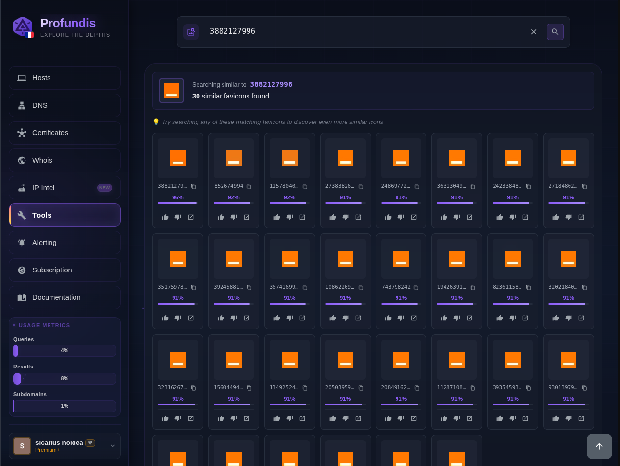
Let’s try some real life examples to show you the power of this new tooling. Keep in mind that the system will always show 30 icons for each query with a given score for each image, even if we don’t have good matches you will see the lower quality ones.

Also, if you want to find all the favicons for your target, do not hesitate to fins the favicons with the lowest score, and try to search for them again to find more related icons with lower quality.

Known icons

Video demo of the system in action

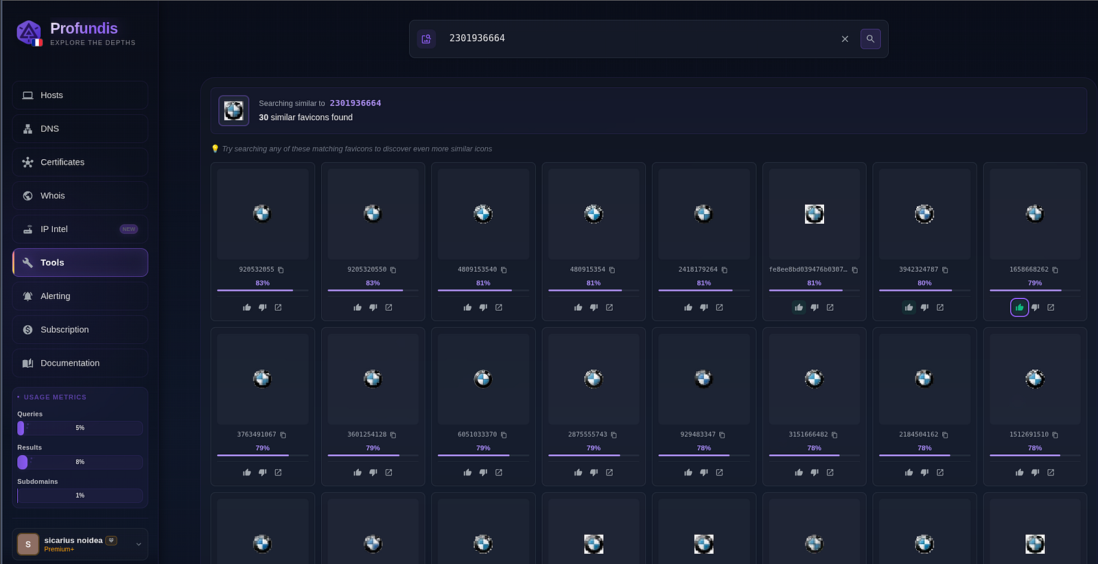
BMW logo, white background

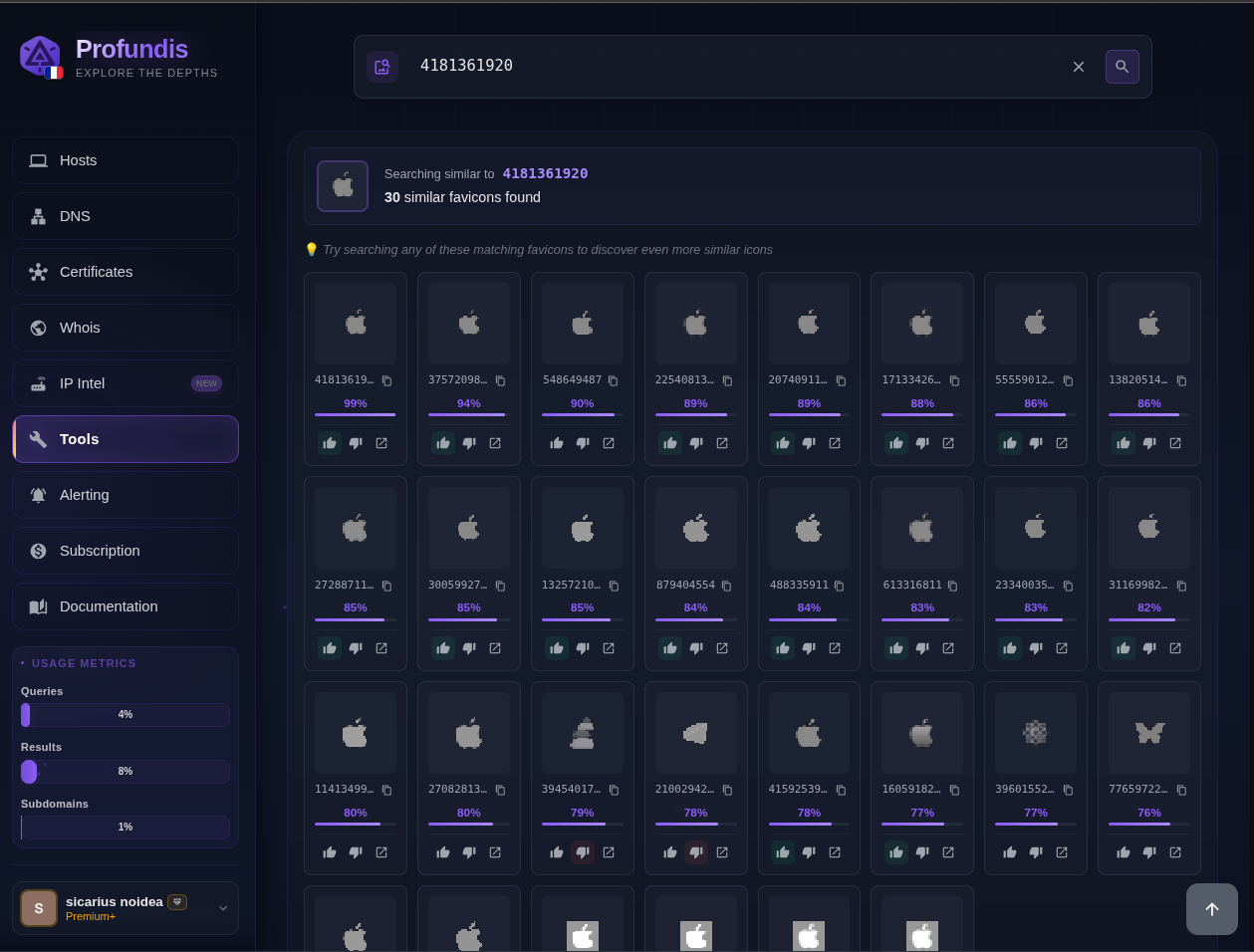
Apple, icon from www.apple.com with a very low quality pixelized logo

First row is a set of icons that looks the same but are slightly different which lead to a different stored hash. The other matches are all round, white background, circular-ish shaped.

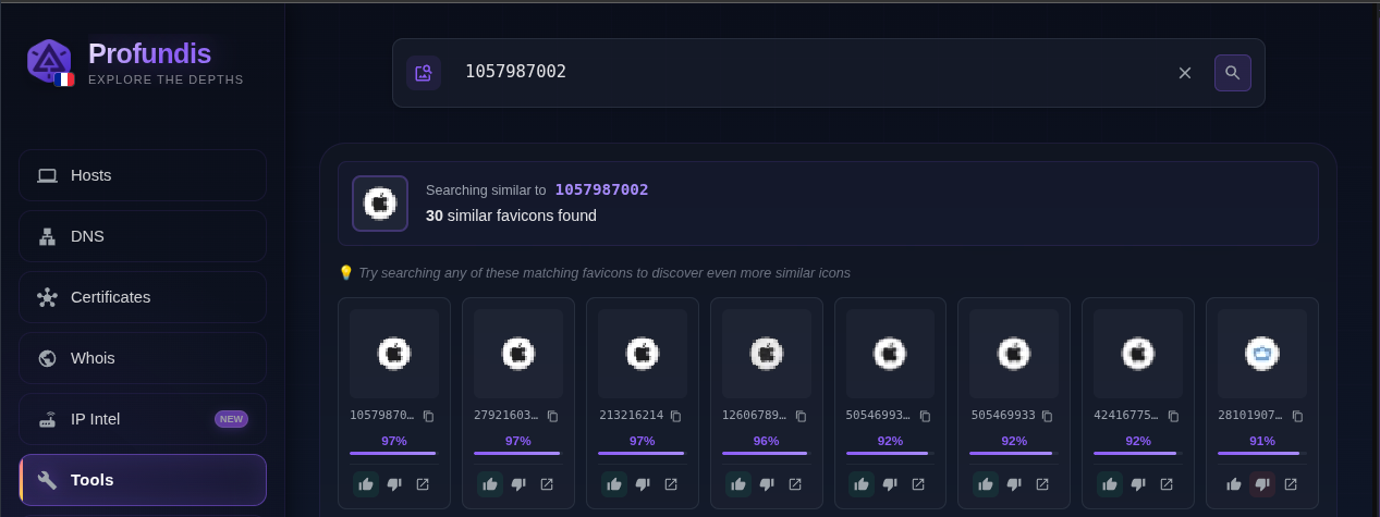
Apple, old grey icon

orange.com, big orange box with a simple white line below:

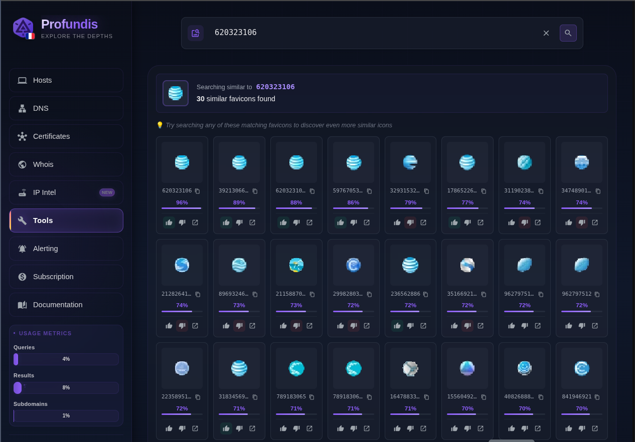
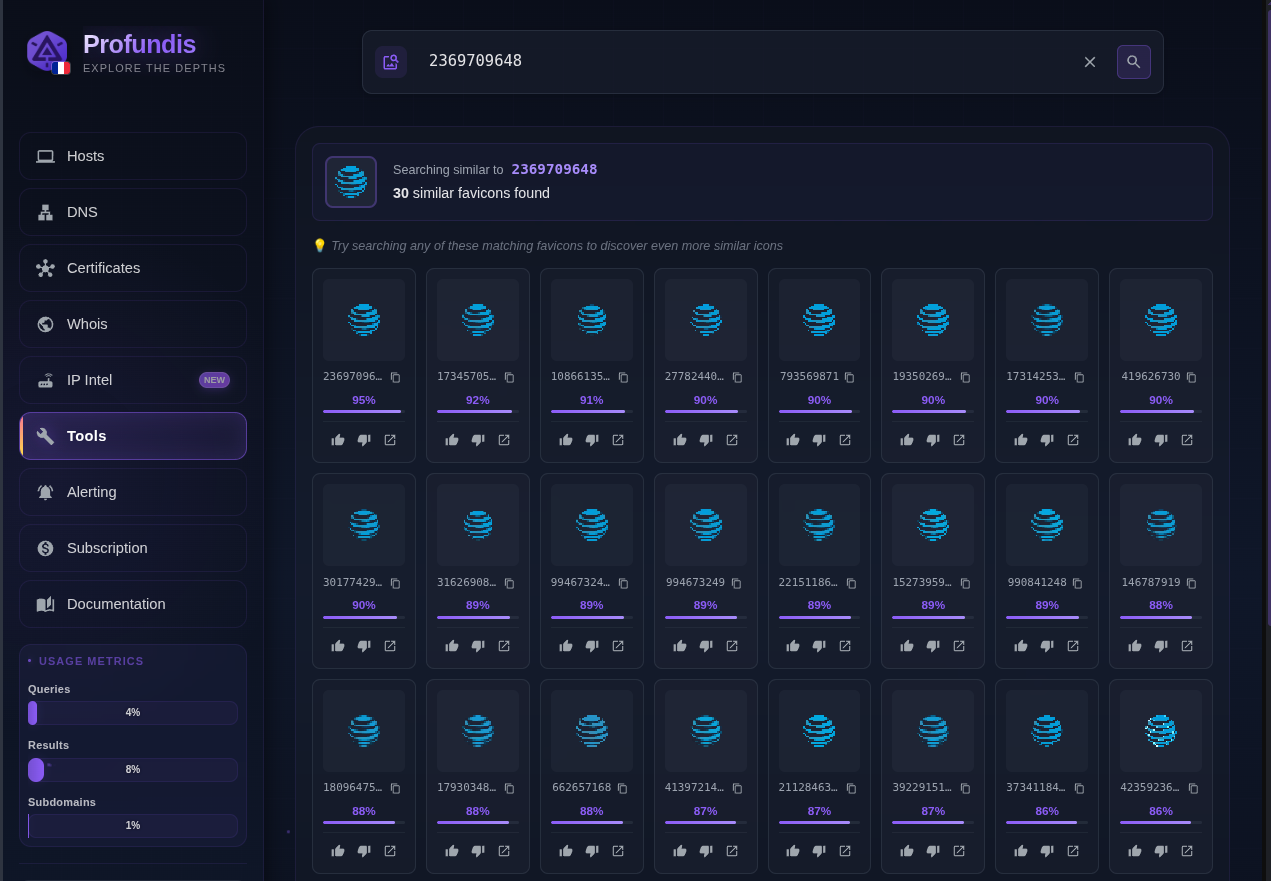
Att.com, blue sphere in low resolution

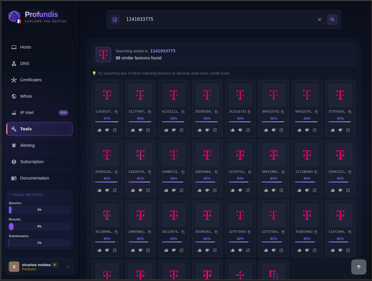
T-mobile.com, letter “T” with dashes round it

Fisglobal.com: A green box with the letters “FIS” and some dots above the “i”

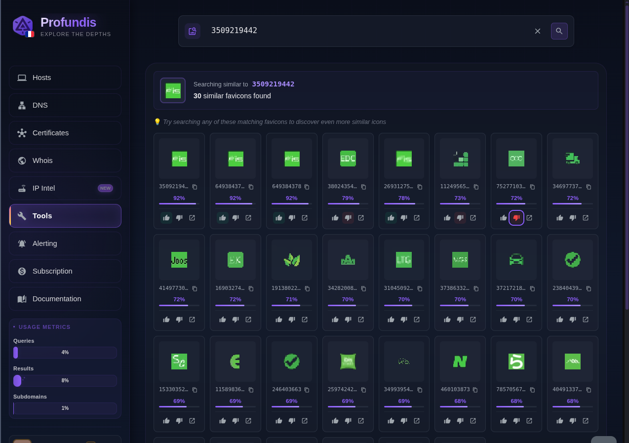This exemple shows that all the relevant results are on top, and less relevant results are following with a starting score of 73% (which is considered bad for our system).

As you can see, we can find related infrastructure only through the favicon!

That’s it for today. I hope you learned something new!

Cheers, Sicarius From the Profundis Team